This article explains in detail the basic theme and need of Genome-wide association studies, the type and format of data we need for it, how we handle, and the tools that perform genome-wide association studies. This is the first part. Then we use the GCTA tool to deliver it a mock example step by step to do GWAS and its visualization.
If you want to learn about the GCTA tool only, scroll down to part 2.
PART 1: Why Genome-Wide Association Studies
Within DNA, there are small variations called Single Nucleotide Polymorphisms (SNPs) — tiny changes at a single base in the sequence. For example, at one position, most people may have an “A,” but some may have a “G.” These SNPs can influence how genes work or how proteins are made.
DNA is the blueprint of life, composed of sequences of four chemical bases: Adenine (A), Thymine (T), Cytosine (C), and Guanine (G). These sequences carry instructions for making proteins, which are essential for all body functions.
Not every SNP causes disease, but some can increase or decrease the risk. For instance, certain SNPs have been linked to higher chances of developing Alzheimer’s or heart disease.
GWAS is a way of scanning hundreds of thousands to millions of these SNPs across many individuals’ genomes. By comparing people with a disease (cases) to those without (controls), GWAS looks for SNPs that appear more often in the cases. These SNPs are considered associated with the disease. That is why it is called a genome-wide association study.
Biologically, this means the variant might:
- Affect gene function or regulation
- Influence protein structure
- Impact gene expression levels
- Be linked to other causative variants nearby
GWAS doesn’t prove causation but highlights regions of interest. Further biological experiments are needed to understand exactly how these variants work.
Importantly, traits can be complex — influenced by many genes and environmental factors. GWAS helps unravel this complexity by identifying multiple genetic contributors.
Statistical Foundations of Genome-wide Association Studies
At its core, GWAS tests the association between each genetic variant (usually SNPs) and the trait or disease status in a large sample of individuals. For each SNP, we ask:
“Is the frequency of this variant different between people with the trait/disease and those without?”
This is a statistical hypothesis test done millions of times, once for each SNP.
1.A. How Data is Built for GWAS – Genotype Data Coding
Genotypes at each SNP are coded numerically for statistical analysis.
- 0 = Homozygous for the reference allele (e.g., AA)
- 1 = Heterozygous (e.g., AG)
- 2 = Homozygous for the alternative allele (e.g., GG)
This numeric coding allows us to use regression models to estimate the effect of each additional copy of the alternative allele on the trait.
1.B. Phenotype Data For GWAS
The phenotype is the trait measured in each individual. It can be:
- Quantitative (continuous), like height or blood pressure.
- Binary (case/control), like presence or absence of disease.
2. Association Testing
For each SNP, GWAS fits a statistical model to test if the genotype predicts the phenotype.
- For quantitative traits, linear regression model is used
3. P-value Calculation for GWAS
After fitting the model, we get a p-value for each SNP’s association. The p-value measures the probability of observing the data assuming there is no real association (null hypothesis).
A low p-value means the variant is unlikely to be unrelated to the trait — suggesting a real genetic association.
4. Multiple Testing and Significance Threshold
Since millions of SNPs are tested, we must account for multiple comparisons to avoid false positives.
This stringent cutoff reduces false positives due to the large number of tests.
The standard genome-wide significance threshold is usually set at p < 5 × 10⁻⁸.
What Data is Needed for GWAS
Performing GWAS requires careful preparation of several types of data files.
1. Genotype Data
- Genotype data contains the genetic variants of each individual.
- Typically stored in formats like:
- PLINK format:
.bed(binary genotype),.bim(variant info),.fam(sample info). - VCF (Variant Call Format): text file listing variants per individual.
- PLINK format:
- Genotype data must cover a large number of SNPs (usually >500,000).
Read about What is PLINK tool?
2. Phenotype Data
- A file listing individuals and their measured traits.
- For example, a CSV with columns: Individual ID, trait value(s), covariates (age, sex).
3. Covariate Data
- Includes factors like sex, age, principal components for population structure.
- Important to adjust for confounding.
4. Sample Metadata
- Information about samples: batch, collection site, ancestry.
5. Reference Genome and SNP Annotation
- To interpret variants, you need reference genome coordinates and annotations (gene locations, known variant effects).
| File Type | Description | Examples |
|---|---|---|
.bed | Binary genotype data | Encodes SNP genotype calls |
.bim | Variant information | SNP IDs, chromosome, position |
.fam | Sample information | Family/individual IDs, sex |
.phen or .csv | Phenotype and covariates | Trait values, covariates |
.vcf | Variant call format | SNP calls with annotations |
.map | SNP position info (older PLINK format) | Chromosome and position |
Popular Tools for Genome-Wide Association Studies
| Tool | Description | Input Files | Output Files | Ease Level | When to Use |
|---|---|---|---|---|---|
| PLINK | Widely used tool for basic GWAS, quality control, filtering, association tests | .bed, .bim, .fam, .phen, .covar | .assoc, .log, summary tables | Easy to Moderate | For quick GWAS, QC, filtering, file conversion |
| GCTA | Estimates SNP-based heritability and mixed model GWAS (GREML, MLMA) | PLINK files + .pheno, .grm, .covar | .hsq, .mlma, log files | Moderate | When estimating heritability or performing mixed model GWAS |
| BOLT-LMM | Fast linear mixed models for large datasets | PLINK files + phenotype + covariates | Association results, logs | Advanced | Large datasets with related individuals/population structure |
| SAIGE | Handles binary traits with imbalanced case-control data | PLINK or VCF + phenotype + GRM + covariates | Association result text file | Advanced | Large case-control studies, especially unbalanced ones |
| GEMMA | GWAS with linear mixed models and Bayesian sparse regression | PLINK or BIMBAM + phenotype + covariates | .assoc.txt, .log, various estimates | Moderate | Mixed models, related individuals, Bayesian modeling |
| SNPTEST | Performs association testing with genotype dosages | .gen or .bgen + .sample, phenotype | Association summary files | Moderate | If working with imputed genotype data |
| HAIL | Python-based framework for scalable GWAS and genomic data analysis | VCF/PLINK/Hail tables | Tables, plots, filtered datasets | Advanced | Very large datasets, cloud-scale analysis |
| REGENIE | Two-step LMM for fast and scalable GWAS, especially binary traits | PLINK files + phenotype + covariates | Text result files, logs | Advanced | High-speed mixed model GWAS on large cohorts |
| GWASpoly | R package for polyploid GWAS (e.g., potato, wheat) | Genotype matrix + phenotype + marker info | R tables, summary plots | Easy to Moderate | When working with polyploid species |
| TASSEL | GUI + CLI software mostly for plant GWAS | HapMap or VCF + phenotype | Tables, plots, visual reports | Beginner-Friendly | Plant breeding GWAS; visual outputs; non-human traits |
How Do We Decide Which SNPs Are Significant in GWAS?
In a GWAS, millions of SNPs (Single Nucleotide Polymorphisms) are tested individually for association with a trait. Each test gives a p-value — the probability that the observed association happened by chance.
But testing millions of SNPs increases the chance of false positives. So, we need to adjust for multiple testing using statistical corrections. This is where methods like Bonferroni Correction and False Discovery Rate (FDR) come in.
Bonferroni Correction (BF Correction)
A very strict method that controls the family-wise error rate — i.e., the probability of making even one false positive.
The idea behind the Bonferroni correction is simple. If you want to keep the overall chance of a false positive at 5%, and you are doing one million tests, then each individual test should only be allowed a p-value of 0.05 divided by one million. That gives a new cutoff of 0.00000005, or 5 × 10⁻⁸. So, after applying Bonferroni, only SNPs with p-values smaller than this extremely tiny number are considered truly significant. This method is very strict. It’s good when you want to be absolutely sure that any SNP you call significant is not a false positive. However, it can be too harsh and might miss some real signals.
When to Use:
- you want to minimize false positives at all costs
- Common in initial GWAS discovery phase
Drawbacks:
- Very conservative — can miss real associations (false negatives)
- Assumes all tests are independent (not always true due to LD)
False Discovery Rate (FDR)
What is it?
FDR controls the expected proportion of false discoveries among all significant results. It’s more lenient than Bonferroni.
Common Method: Benjamini-Hochberg Procedure
The FDR method, particularly the Benjamini-Hochberg procedure, works by first arranging all the p-values from your GWAS in order, from smallest to largest. Each p-value is then compared to a calculated threshold that depends on its position in the list (its rank), the total number of tests, and the desired FDR level (for example, 5%). If a SNP’s p-value is smaller than this threshold, it is marked as significant. What’s clever about this method is that it gives more leniency to lower-ranked p-values (the most promising ones) and becomes stricter as it moves down the list. This method lets researchers identify more potentially interesting SNPs while still keeping the expected proportion of false positives under control.
When to Use:
- When you’re okay with a small % of false positives
- In exploratory GWAS or follow-up analysis
- For polygenic traits with many small-effect SNPs
Visualization of GWAS
Visualizing the results of genome-wide association studies (GWAS) is a crucial step for interpreting and communicating findings. Raw statistical outputs from GWAS can be overwhelming due to the massive number of genetic variants tested, often in the millions. Effective visualization helps researchers quickly identify significant associations, understand the genetic architecture of traits, and detect potential artifacts or biases.
Why Visualize GWAS Results?
- Identify Significant SNPs Quickly
GWAS tests millions of single nucleotide polymorphisms (SNPs) across the genome. Visualization allows pinpointing variants with strong statistical evidence for association with the trait of interest. - Explore Genomic Regions of Interest
Visual tools enable zooming into specific chromosomes or gene regions to inspect the pattern of association and linkage disequilibrium. - Detect Potential Confounding and Bias
Some visualizations can reveal issues like population stratification, cryptic relatedness, or batch effects that might inflate false positives. - Communicate Results Clearly
Well-designed plots are essential for publications and presentations, making complex data accessible to diverse audiences.
Common Plots for GWAS Visualization
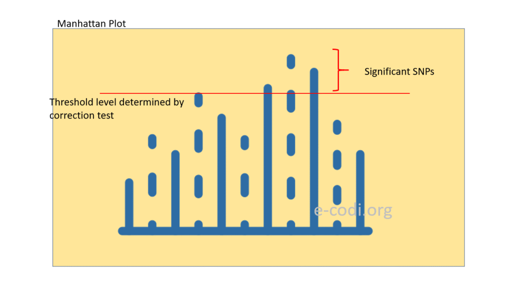
1. Manhattan Plot
- What It Shows:
A Manhattan plot displays the negative logarithm of the p-value (−log10 p) for each SNP tested, plotted against its genomic position, typically ordered by chromosome and base pair position. - Purpose:
Peaks represent SNPs strongly associated with the trait. The higher the peak, the more significant the association. - Features:
- Chromosomes often colored alternately for clarity.
- A horizontal line indicates the genome-wide significance threshold (e.g., p < 5×10⁻⁸).
- Clusters of SNPs in high linkage disequilibrium can appear as a “skyline” over a genomic region.
- Interpretation:
Helps identify candidate loci and assess whether associations are clustered or isolated.
2. Quantile-Quantile (QQ) Plot
- What It Shows:
QQ plots compare the distribution of observed GWAS p-values to the expected distribution under the null hypothesis (no association). - Purpose:
To assess if there is an inflation of test statistics (which might indicate population stratification or technical artifacts) or true signals. - Features:
- Points falling along the diagonal indicate observed p-values match expected.
- Upward deviation at the tail suggests significant associations.
- Systematic inflation (deviation along the whole range) signals potential confounding.
- Interpretation:
Helps evaluate the overall quality and validity of GWAS results.
Additional Visualization Techniques
- Manhattan plots with effect sizes: Show direction and magnitude of SNP effects alongside p-values.
- Forest plots: Display effect estimates and confidence intervals for top SNPs across multiple studies or cohorts.
- Heatmaps: Used to display linkage disequilibrium or gene expression correlations.
- Circos plots: Visualize complex relationships such as inter-chromosomal interactions or multi-trait associations.
Tools for GWAS Visualization
Several software tools and packages can create publication-quality visualizations:
- R packages:
qqman: Simple Manhattan and QQ plots.LocusZoom: For regional association plots.ggplot2: Flexible general plotting framework for custom visualizations.
- Python libraries:
matplotlibandseabornfor custom plots.PyLocusZoomfor regional plots.
PART 2: Step-by-step Example: GWAS Using GCTA with Mock Data
1. What Files Are Needed?
For GCTA GWAS (using a simple mixed linear model association – MLMA), you need mainly:
| File Type | File Extension(s) | What It Contains |
|---|---|---|
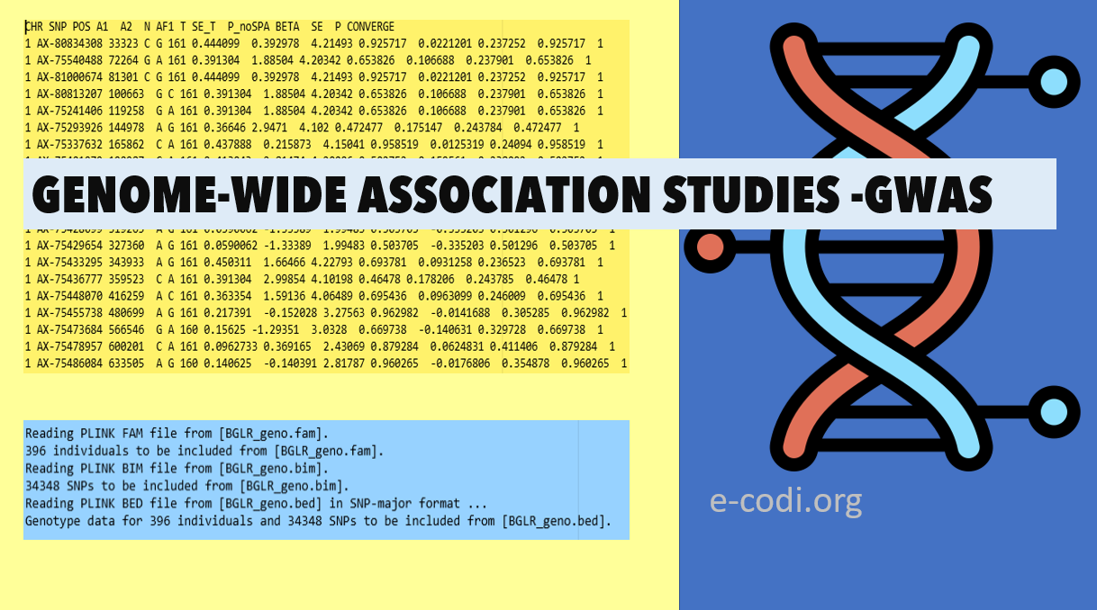
| Genotype Data | .bed, .bim, .fam | SNP genotype data in PLINK binary format |
| Phenotype File | .pheno or .txt | Sample IDs + phenotype values |
| Covariate File | .covar or .txt | Sample IDs + covariates (optional) |
| Genetic Relationship Matrix (GRM) | .grm, .grm.id (optional if calculated) | Pairwise relatedness between individuals (used for mixed model) |
2. Mock Example Data
Genotype files (PLINK binary format)
.bed: binary genotype data.bim: SNP info (chromosome, SNP ID, position, alleles).fam: sample info (family ID, individual ID, father, mother, sex, phenotype)
These are usually generated or obtained from real genotype data using PLINK.
For simplicity, imagine we have mock.bed, mock.bim, and mock.fam.
Phenotype file: mock.pheno
FID     IID     Trait
FAM1    IND1    2.5
FAM1    IND2    3.7
FAM2    IND3    1.9
FAM2    IND4    4.1
...
FID: Family IDIID: Individual IDTrait: Quantitative phenotype (e.g., height, weight, blood pressure)
3. Preparing Data
- Make sure
.bed,.bim,.famare in the same folder. - Phenotype file is a simple tab-delimited text file with header.
4. Tools Needed
- PLINK: To prepare genotype data if needed (optional)
- GCTA software: For GWAS and heritability analysis -download the latest version
- Terminal or Command Prompt: To run commands (R Studio terminal for example)
- R: For downstream data visualization (optional)
What is GCTA-MLMA & GCTA-LOCO for GWAS analysis?
What is MLMA?
MLMA stands for Mixed Linear Model Association — a method in GCTA (Genome-wide Complex Trait Analysis) used to perform GWAS while accounting for population structure and relatedness among individuals.
In standard GWAS, population structure (like ancestry differences) can lead to false positives. MLMA uses a linear mixed model that adds a random effect (polygenic effect) to control for this structure.
LOCO – Leave One Chromosome Out
When using MLMA, if the SNP being tested is also used to calculate the GRM, it may create bias or inflation.
LOCO solves this by excluding the chromosome that contains the SNP being tested from the GRM.
LOCO is used in following conditions
- When sample size is large
- When testing SNPs on each chromosome
- To avoid proximal contamination (SNPs helping explain themselves)
How to Run GCTA GWAS: Step by Step
Step 1: Calculate Genetic Relationship Matrix (GRM)
This is needed for the mixed model to account for relatedness.
gcta64 --bfile mock --make-grm --out mock_grm
--bfile mocktells GCTA to use PLINK binary files namedmock.bed,mock.bim,mock.fam.--make-grmcalculates the GRM.--out mock_grmspecifies output prefix.
This produces mock_grm.grm.bin, .grm.N.bin, .grm.id.
You can select two types of types while doing GWAS by GCTA
1. Gaussian (Continuous) Response
These are quantitative traits like height, weight, blood pressure.
MLMA assumes normal distribution and works perfectly with these.
→ Use MLMA directly for these traits.
2. Ordinal Traits (e.g., pain level: none, mild, moderate, severe)
GCTA does not natively support ordinal categorical traits. However, you can:
Option 1: Treat Ordinal as Continuous
- Assign numbers (e.g., 0, 1, 2, 3)
- Use MLMA assuming a Gaussian approximation
- Works best when categories have linear meaning
Option 2: Use Other Tools Like:
- SAIGE: Can model binary and ordinal outcomes with correction for relatedness
- GEMMA: For more complex models, including probit/logistic regression
- BOLT-LMM: Fast for large datasets, mostly for continuous traits
Step 2: Run GWAS with Mixed Linear Model (MLMA)
gcta64 --bfile mock --grm mock_grm --pheno mock.pheno --mlma --out mock_gwas


it could be also like this

gcta64 --mlma-loco \
       --grm mydata \
       --pheno phenotype.txt \
       --qcovar covariates.txt \
       --out gwas_results
--bfile mock: genotype files--grm mock_grm: the GRM calculated before--pheno mock.pheno: phenotype file--mlma: run mixed linear model association--out mock_gwas: output prefix
6. Output Files
mock_gwas.mlma: association results with SNP, chromosome, position, effect size, p-value, etc.mock_gwas.log: log file with command output and statistics.
7. Interpreting Results
Open the .mlma file in Excel, R, or any text editor. Columns include:
- SNP ID
- Chromosome
- Position
- Allele info
- Effect size (beta)
- Standard error
- p-value
Look for SNPs with very small p-values (e.g., < 5×10⁻⁸) as significant hits.
8. Running Commands in Terminal or R Terminal
system("gcta64 --bfile mock --make-grm --out mock_grm")
system("gcta64 --bfile mock --grm mock_grm --pheno mock.pheno --mlma --out mock_gwas")
9. Simple R Code to Load and Plot GWAS Result
#Load GWAS result
gwas_res <- read.table("mock_gwas.mlma", header=TRUE)

# Manhattan plot (basic)
library(ggplot2)

gwas_res$logp <- -log10(gwas_res$P)

ggplot(gwas_res, aes(x=BP, y=logp, color=as.factor(CHR))) +
  geom_point(alpha=0.6) +
  scale_color_manual(values = rep(c("blue", "red"), max(gwas_res$CHR))) +
  theme_minimal() +
  labs(title="Mock GWAS Manhattan Plot", x="Position (bp)", y="-log10(p-value)") +
  theme(legend.position = "none")
Genome-Wide Association Studies (GWAS) have become an indispensable tool in modern genetics, allowing researchers to pinpoint genetic variants linked to complex traits and diseases. From identifying risk loci in human diseases to uncovering behavioral traits in animals and plants, GWAS empowers scientists to unlock the genetic blueprint like never before.
In this guide, we broke down GWAS in simple, beginner-friendly terms—starting from what it is, how it works biologically, and how it’s applied statistically. You’ve seen how statistical models like linear regression analyze millions of SNPs, and how significance is determined through stringent corrections like the Bonferroni method and FDR. We also explored the essential data formats used in GWAS, the role of phenotype and genotype files, and demonstrated how to conduct a basic GWAS using real commands via GCTA software in R.
Whether you’re just stepping into the world of genomics or refining your bioinformatics pipeline, GWAS offers a powerful way to associate genetic variation with observable traits. With tools like PLINK, GCTA, and GEMMA at your disposal, and visualizations like Manhattan plots and QQ plots to guide interpretation, you’re equipped to generate insights from DNA that can shape future research, medicine, and breeding programs.
If you’re serious about mastering GWAS, continue exploring statistical genetics, ensure proper data quality control, and stay up to date with the latest GWAS methodologies. The genome has stories to tell—GWAS is your microphone.