PLINK Files & Commands – A Complete Guide

What is PLINK?

PLINK is a computer program that helps scientists study DNA data. It is used mostly in something called genome-wide association studies (GWAS). That means scientists try to find out how certain parts of DNA are related to diseases, traits like height or eye color, or other biological information.

Think of PLINK as a super-powered calculator that can understand genetics.

Why Is It Called PLINK?

The name PLINK doesn’t stand for anything fancy—it’s just a simple, catchy name chosen by its creator, Shaun Purcell. It reflects a lightweight, fast tool designed to “plink” through your genome data.

If you’re working with genomic data—for example, from a genotyping array or whole-genome sequencing—you’ll need a tool to clean, filter, and analyze that data. One of the most widely used tools is PLINK. It’s a command-line program designed for fast, flexible, and memory-efficient genetic data analysis.

How Is Biological Data Created for PLINK?

Let’s say a group of scientists wants to study what makes some people taller than others. First, they gather samples from people: usually saliva or blood. These samples go to a genotyping lab, where machines read their DNA.

These machines break the DNA into SNPs (Single Nucleotide Polymorphisms), which are small differences in DNA. Each person’s DNA has millions of these SNPs.

What Kind of Files Does PLINK Use?

PLINK reads data from different file formats. The most common are:

PED file (.ped)	A text file with information about each person and their genotypes.
MAP file (.map)	Tells PLINK where each SNP is located in the genome.
BED file (.bed)	Binary file storing the genotype data (compressed form).
BIM file (.bim)	Like .map, but for the binary version.
FAM file (.fam)	Like .ped, but for the binary version.

What Does Each File Contain?

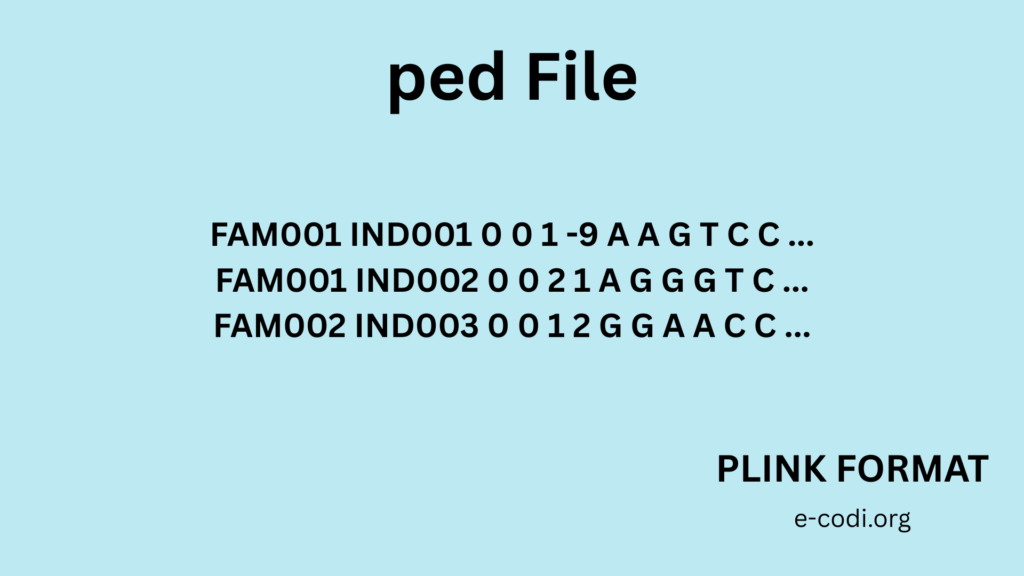
1. PED File Format

It is a space- or tab-delimited file. Each row is one person.

Columns:

Family ID
Individual ID
Paternal ID (father)
Maternal ID (mother)
Sex (1 = male, 2 = female)
Phenotype (1 = unaffected, 2 = affected) 7+. Genotype data (like A T, G C for each SNP)

2. MAP File Format

Each line is one SNP.

Columns:

Chromosome number (1, 2, … X, Y)
SNP ID
Genetic distance (can be 0)
Base-pair position

3. FAM File Format

Like the first 6 columns of PED:

Family ID
Individual ID
Paternal ID
Maternal ID
Sex
Phenotype

4. BIM File Format

Like the MAP file, but with a bit more info:

Chromosome
SNP ID
Genetic distance
Base-pair position
Allele 1
Allele 2

5. BED File Format

Stores genotypes in a compact format. It’s not human-readable, but very fast for computers.

Where Can Problems Happen?

Even though PLINK is great, problems can occur:

Missing values: If someone forgot to type in an ID or genotype.
Incorrect sex info: Someone typed 1 instead of 2.
File mix-up: Using a PED with a wrong MAP file.
Non-matching SNPs: Different files report different numbers of SNPs.
Corrupted files: Especially BED files if saved incorrectly.

Where Do You Run PLINK Commands?

To run PLINK commands, you need a Unix-like terminal environment (Linux or macOS) or the Windows command prompt (or better, Git Bash or WSL on Windows). PLINK is a command-line tool, meaning there’s no graphical interface — you use text commands to interact with your data.

1. Install PLINK

On Linux/macOS:
Download the binary from https://www.cog-genomics.org/plink/ and unzip it into a folder, e.g., ~/tools/plink/. Make it executable with chmod +x plink and add it to your PATH.
On Windows:
Download the .zip file, extract it, and either run commands from the folder or add it to the system PATH. You can use:
- Command Prompt
- PowerShell
- Better: Git Bash or Windows Subsystem for Linux (WSL)

🖥️ 2. Where You Run Commands

You open a terminal or command prompt, cd (change directory) into your working folder — where your .bed, .bim, .fam, or .ped/.map files are located — and then run PLINK commands

What is PLINK Used For?

Before Starting

Before any analysis can begin, it’s important to understand what kind of data PLINK expects.

The most common input formats are PED/MAP and BED/BIM/FAM.

PED and MAP files are simple text files: the .ped file contains sample and genotype information for each individual, while the .map file contains SNP information such as chromosome, position, and ID.

However, for efficient processing, PLINK prefers its binary format consisting of three files: .bed (binary genotype data), .bim (variant information), and .fam (sample information).

If your data is in .ped and .map format, you’ll need to convert it to binary format using the command plink --file data --make-bed --out dataset.

This tells PLINK to read data.ped and data.map, convert them to .bed, .bim, and .fam, and save them under the name dataset. This step is crucial because most downstream PLINK commands work only with the binary format, which is significantly faster and smaller in size.

🔹 1. Quality Control (QC)

This is perhaps the most critical stage in genomic analysis, as poor-quality data can easily lead to false conclusions. The QC process involves several filtering steps. Quality control has four major steps using PLINK.

First, you remove SNPs (genetic markers) that have a high proportion of missing values using the command plink --bfile dataset --geno 0.05 --make-bed --out qc_step1. This excludes all SNPs missing in more than 5% of individuals, which could indicate technical errors or poorly designed assays.
After filtering bad SNPs, the next step is to remove individuals (samples) who have a high rate of missing genotypes. This is done with plink --bfile qc_step1 --mind 0.05 --make-bed --out qc_step2, which removes any individual with more than 5% missing data. These low-quality samples can skew your results, especially in small studies.
Once both SNPs and individuals are cleaned for missing data, you filter out rare variants using the minor allele frequency (MAF). This is usually done with plink --bfile qc_step2 --maf 0.01 --make-bed --out qc_step3, which retains only those SNPs where the less common allele is present in at least 1% of individuals. Rare variants can be useful in some studies but are often excluded in general GWAS to reduce noise and false positives.
Another essential QC step is filtering based on Hardy-Weinberg Equilibrium (HWE). SNPs that deviate significantly from HWE might indicate genotyping problems or population stratification. You can remove such SNPs with plink --bfile qc_step3 --hwe 1e-6 --make-bed --out qc_final, which excludes markers with a p-value less than 1e-6 in HWE tests.

Common QC steps include:

plink --bfile data --geno 0.05 --make-bed --out step1
plink --bfile step1 --maf 0.01 --make-bed --out step2
plink --bfile step2 --hwe 1e-6 --make-bed --out final_data

Remove SNPs with missing genotypes (--geno)
Remove rare SNPs by minor allele frequency (--maf)
Hardy-Weinberg equilibrium filtering (--hwe)

🔹 2. Association Studies (GWAS)

If your phenotype is binary (e.g., case vs. control), and you have a file called phenotype.txt listing each sample’s phenotype, you can run a basic association test using plink --bfile data_pruned --pheno phenotype.txt --assoc --out assoc_results. This performs a chi-squared test for each SNP and saves the p-values in assoc_results.assoc. Tests SNPs for association with a phenotype.

plink --bfile dataset --pheno phenotype.txt --assoc --out assoc_results

Case-control or quantitative trait association
Logistic (--logistic) or linear regression (--linear)

🔹 3. Linkage Disequilibrium (LD) Analysis

Check SNP correlation or prune SNPs in LD.

plink --bfile dataset --r2 --ld-snp rs123 --ld-window 100 --out ld_output
plink --bfile dataset --indep-pairwise 50 5 0.2 --out pruned

Used for fine-mapping or reducing redundancy

🔹 5. Genotype Imputation Preparation

Prepares files for imputation services (e.g., Michigan, Sanger, TOPMed).

plink --bfile dataset --recode vcf --out output

Converts to VCF for imputation
Can also phase with SHAPEIT or Eagle and impute externally

🔹 6. Relationship & Kinship Analysis

Estimate relatedness between individuals.

bashCopyEditplink --bfile dataset --genome --out kinship

Outputs IBS and IBD coefficients (pi-hat)
Useful to detect duplicates, relatives, or sample swaps

🔹 7. Genetic Risk Score (GRS) / PRS

Calculate polygenic risk scores (PRS) using SNP weights.

bashCopyEditplink --bfile genotype --score weights.txt 1 2 3 --out prs

weights.txt: SNP ID, allele, effect size
Used in disease prediction models

🔹 8. Data Conversion

PLINK supports many formats:

bashCopyEditplink --bfile input --recode --out text_data
plink --bfile input --recode vcf --out data_vcf

Convert between:

BED ↔ PED/MAP
BED ↔ VCF
BED ↔ RAW
PED ↔ VCF

PLINK Files Are the Foundation for Many Tools

While PLINK is a powerful standalone tool for conducting genome-wide association studies (GWAS), its importance goes beyond just running commands in PLINK itself. In fact, many advanced tools in statistical genetics rely on PLINK-formatted files as input, especially tools like GCTA (Genome-wide Complex Trait Analysis), which is widely used for estimating heritability, performing GREML (genomic REML), and running mixed linear models.

GCTA

GCTA specifically requires PLINK binary files (.bed, .bim, .fam) as input. These files contain genotype information (.bed), SNP/variant information (.bim), and individual/sample information (.fam). So even if you’re not performing your actual GWAS in PLINK (e.g., you’re using GCTA or BOLT-LMM or SAIGE), you’ll often need to start your data processing and QC in PLINK, then pass the cleaned dataset to GCTA.

For example, once you’ve completed all quality control steps in PLINK and created a clean binary dataset (say, qc_final.bed, qc_final.bim, qc_final.fam), you can run a GCTA heritability estimation using:

gcta64 --bfile qc_final --make-grm --out myGRM
gcta64 --grm myGRM --pheno phenotype.txt --reml --out heritability_results

Other Tools

Another widely-used tool is BOLT-LMM, which is designed to handle large-scale GWAS using linear mixed models efficiently. Like GCTA, BOLT-LMM accepts PLINK-format genotype data (.bed, .bim, .fam) for running population-scale association tests, especially on datasets like the UK Biobank.

PLINK files are also crucial for PRSice (Polygenic Risk Score software), which calculates polygenic risk scores based on GWAS summary statistics and individual genotype data. PRSice reads PLINK files to calculate individual-level risk profiles using scoring methods that account for linkage disequilibrium (LD) and variant weights.

Additionally, PLINK-formatted data is used in LDPred2 and SBayesR, tools that perform LD-adjusted risk score prediction and Bayesian modeling, respectively. They often require a PLINK-formatted LD reference panel or training set, emphasizing how PLINK outputs form the foundation for high-level statistical modeling.

In the realm of population structure and stratification, PLINK files are used in ADMIXTURE, a fast maximum likelihood estimation tool that estimates individual ancestry proportions. ADMIXTURE reads PLINK .bed files directly to model ancestries and produce Q matrices.

Furthermore, IMPUTE2, Beagle, and SHAPEIT—commonly used for genotype imputation and phasing—either accept PLINK files directly or require conversion from them via intermediate tools like plink2 or convert.

Even popular data visualization and QC tools like Hail, SNPRelate, and GenABEL in R can read PLINK files or convert them into internal formats for exploration and downstream analysis.

What makes PLINK file formats so ubiquitous is their efficiency, compatibility, and compact structure. The .bed file stores genotype information in a compressed binary form, while .bim and .fam store SNP and sample metadata. These formats offer a consistent, easy-to-parse structure that has become a universal language in genomic computing.