Biological data integration means combining different kinds of biological data into a single framework so you can make more meaningful conclusions.
These datasets may include genomic data (such as DNA sequences), transcriptomic data (gene expression levels), proteomic data (information on protein presence and activity), phenotypic data (observable physical or behavioral traits), metabolomic data (metabolic activity and chemical processes), and environmental data (such as microbiome composition or exposure to external factors).
Instead of analyzing each data type in isolation, researchers use specialized software, algorithms, and biological databases to merge these datasets, enabling a more comprehensive and interconnected view of biological functions and interactions. This holistic approach is crucial in areas like disease research, personalized medicine, and systems biology, where understanding the full picture can lead to more accurate insights and meaningful conclusions.
It helps you see how one layer of biology affects another.
You don’t need to be a data scientist to start understanding this. Whether you’re a plant biologist, veterinarian, or someone working with cell cultures or ecosystems—this guide is for you.
This article has three parts
- PART 1 – Understanding data integration and type of data
- PART 2 – Example codes and tools for various type of data integration
- PART 3 – Challenges in Data integration in biology

It’s like understanding the relationship between:
- A genetic mutation and a disease symptom.
- A microbial imbalance and plant growth.
- A behavioral change and a metabolic shift.
Instead of just looking at one layer (like just genes), we use multiple data types together—DNA, RNA, proteins, environments, phenotypes, etc.—to get a full picture.
This is sometimes called:
- Integrative biology
- Biological data fusion
- Multi-omics analysis
- Cross-platform analysis
- Integrated life science research
What Kinds of Data Do We Collect in Biology?
Modern biology generates many different kinds of data. Here are the main categories, plus real-world examples:
1. Genotype Data
- What it is: DNA sequences, SNPs, mutations.
- Examples: Human genome, plant SNPs, CRISPR edits.
- Format: VCF, FASTA, PLINK binary (
.bed,.bim,.fam)
2. Phenotype Data
- What it is: Observable traits—height, disease resistance, flower color.
- Examples: Biomass, cholesterol levels, survival under stress.
- Format: CSV or Excel tables, often with rows = individuals, columns = traits.
3. Time-Series Data
- What it is: Repeated measurements across time.
- Examples: Gene expression over time, response to drug treatment.
- Format: Tabular or matrix-style data; often used in longitudinal studies.
4. Microbiome Data
- What it is: Which microbes live in a sample and in what amounts.
- Examples: Gut microbiome, soil rhizosphere bacteria.
- Format: OTU/ASV tables, metadata, usually from 16S or metagenomic sequencing.
5. Behavioral Data
- What it is: Observable behaviors recorded over time or per event.
- Examples: Mating behavior in insects, feeding rates, movement tracking.
- Format: Time-stamped logs, video analysis outputs, scores.
6. Biochemical or Molecular Data
- What it is: Protein levels, metabolites, enzymes, pathway activity.
- Examples: Mass spectrometry, ELISA, NMR data.
- Format: CSV matrices, tables, often with annotations.
7. Environmental and Location Data
- What it is: Conditions that affect the organism.
- Examples: Soil moisture, GPS location, light levels, pH.
- Format: Sensor logs, geographic data (GeoTIFF, shapefiles), metadata spreadsheets.
PART 2: How Is Data Integration Done in Biology?
Let’s now walk through practical examples of data integration across different biological data types using one common approach per case—with simple R code snippets you can try.
1. Genotype + Phenotype Integration: GWAS Using PLINK in R
One of the most common types of biological data integration is connecting genetic variants (SNPs) with observable traits like height or disease resistance. This is the basis of a Genome-Wide Association Study (GWAS).
We’ll use PLINK and R to perform this integration.
Example Files
data.bed, data.bim, data.fam – your SNP data – [Learn PLINK and its files in detail here]
pheno.txt – phenotype file
# Run a PLINK-based GWAS from within R

# Step 1: Call PLINK command-line tool to perform association analysis
# --bfile: base name of your PLINK binary files (data.bed, data.bim, data.fam)
# --pheno: the file containing phenotype data
# --assoc: request basic association test
# --out: name of the output file

system("plink --bfile data --pheno pheno.txt --assoc --out gwas_result")

# Step 2: Read the resulting association results back into R
# This file contains SNP IDs, allele frequencies, effect sizes, and p-values
gwas <- read.table("gwas_result.assoc", header = TRUE)

# Step 3: View the top SNP associations
head(gwas)
2. Time-Series + Gene Expression Integration: DESeq2 for RNA-seq over Time
Let’s say you have gene expression data collected over multiple time points and want to see how it changes under treatment vs. control.
We use DESeq2 for time-aware differential analysis.
# Install if needed the package DESeq2 In R studio
if (!require("DESeq2")) install.packages("BiocManager"); BiocManager::install("DESeq2")

library(DESeq2)  #for loading pacakge

# Simulated gene expression counts
# 100 genes (rows), 3 samples (columns)

counts <- matrix(sample(1:1000, 300, replace = TRUE), nrow = 100)
colnames(counts) <- paste0("sample", 1:3)  # Names like sample1, sample2, sample3
rownames(counts) <- paste0("gene", 1:100)  # Simulated gene IDs like gene1, gene2, ...


# Metadata (the file containing time situtaion of each sample)
colData <- data.frame(
  time = factor(c("0h", "2h", "6h")),
  treatment = factor(c("control", "treated", "treated"))
)
rownames(colData) <- colnames(counts)

# Create and run DESeq
dds <- DESeqDataSetFromMatrix(countData = counts, colData = colData, design = ~ time + treatment)
dds <- DESeq(dds)
results <- results(dds)
head(results)
Microbiome + Trait Data Integration with Phyloseq
What This Data Represents:
- Microbiome data: Microbial composition of samples (e.g., gut or soil bacteria).
- Trait data: Measured traits like pH, weight, or inflammation score
library(phyloseq)

# Load example microbiome dataset (includes OTUs, taxonomy, metadata)
data(GlobalPatterns)

# Calculate Shannon diversity for each sample
# Shannon index = measure of microbial diversity (higher = more diverse)
shannon <- estimate_richness(GlobalPatterns, split = TRUE, measures = "Shannon")

# Attach Shannon diversity back into sample metadata
sample_data(GlobalPatterns)$Shannon <- shannon$Shannon

# Example: correlate pH of the environment with microbial diversity
plot(sample_data(GlobalPatterns)$pH, sample_data(GlobalPatterns)$Shannon,
     xlab = "pH", ylab = "Shannon Diversity")
abline(lm(sample_data(GlobalPatterns)$Shannon ~ sample_data(GlobalPatterns)$pH), col = "blue")
Multi-Omics Fusion with MOFA2
- Multiple omics layers for the same individuals:
data1: gene expressiondata2: metabolite profiles
Each matrix: rows = individuals, columns = variables (e.g., genes or metabolites)
library(MOFA2)

# Simulate omics data (e.g., gene expression and metabolomics)
data1 <- matrix(rnorm(100*50), nrow = 100)  # 100 samples, 50 genes
data2 <- matrix(rnorm(100*30), nrow = 100)  # 100 samples, 30 metabolites

# Combine them into a list
data_list <- list(omics1 = data1, omics2 = data2)

# Initialize MOFA object with your multi-layer data
mofa <- create_mofa(data_list)

# Set default model and training options
model_opts <- get_default_model_options(mofa)
train_opts <- get_default_training_options()

# Run MOFA model training
trained_model <- run_mofa(mofa)

# The trained model now captures **shared latent patterns** between gene and metabolite layers
Behavior + Biochemistry with MixOmics
What This Data Represents:
Y = Behavioral scores, like memory test results, movement speed, or feeding behavior.
X = Biochemical data, like protein or metabolite levels from a mass-spec.
install.packages("mixOmics")
library(mixOmics)

# Simulate protein/metabolite levels for 100 samples across 20 features
X <- matrix(rnorm(100*20), nrow = 100)

# Simulate behavioral scores (like learning speed, activity level) across 5 behaviors
Y <- matrix(rnorm(100*5), nrow = 100)

# Perform partial least squares (PLS) regression to find relationships
result <- pls(X, Y, ncomp = 2)

# Visualize samples in the latent space (shared behavior-biochemistry space)
plotIndiv(result, group = rep(c("Group1", "Group2"), each = 50))
Key Points
- Use PLINK or
GWASpolyfor genotype-phenotype integration. - Use DESeq2 for time-series transcriptomics.
- Use phyloseq + vegan for microbiome + trait studies.
- Use MixOmics for behavioral + molecular data.
- Use MOFA2 for multi-omics fusion.
No matter which domain you’re in—plants, animals, microbes, or humans—these tools can help you integrate biological datasets to find insights that wouldn’t be visible from any one layer alone.
PART 3: Challenges in Biological Data Integration

While integrating biological data opens new doors for discovery, it’s not always easy. Many challenges can affect how reliable, meaningful, or interpretable the integrated data is. Ignoring these issues can lead to false conclusions or missed insights.
Let’s go through the major challenges and how to deal with them—especially if you’re a biologist working without formal data science training.
Incompatible Data Formats and Structures
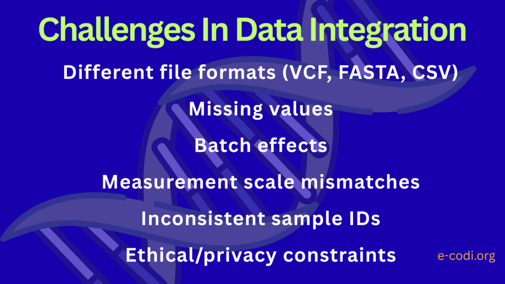
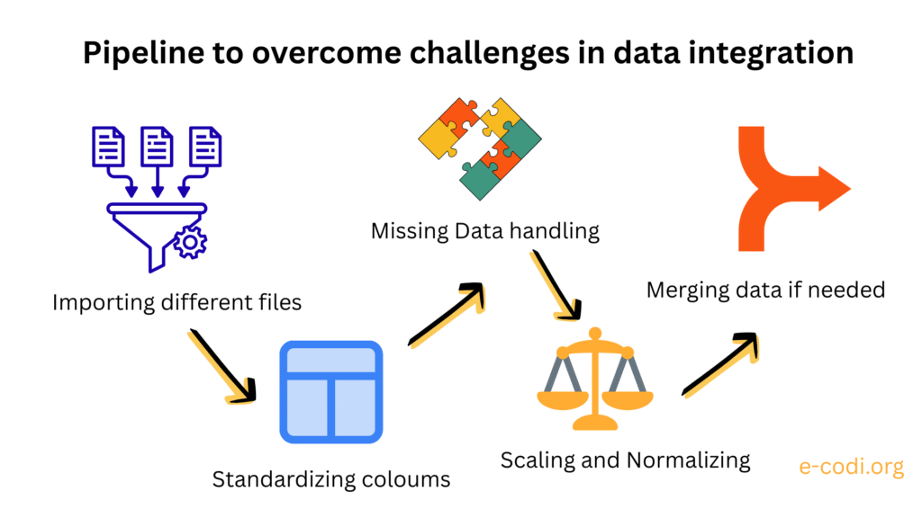
One of the first problems researchers encounter in data integration is the mismatch in data formats. Biological data is incredibly diverse—not just in content, but in structure. Genetic data might come in VCF files, gene expression in matrices of count values, and microbial community data as OTU tables. Phenotypic records might be in CSV files or handwritten logs, each with slightly different naming conventions, separators, and metadata fields. For example, one dataset might label samples as Sample_01, while another calls them S1. Even minor inconsistencies like this can prevent automated merging or alignment of data, leading to wasted time and inaccurate conclusions. To integrate these datasets meaningfully, they first need to be cleaned, harmonized, and sometimes reshaped into a common structure—often a “long” or “tidy” format preferred by statistical tools in R or Python.
Differences in Scale and Measurement Units
Once formats are aligned, the next hurdle is dealing with different types of measurements. Imagine you’re combining leaf width in centimeters, soil nitrogen concentration in parts per million, and gene expression in log2-transformed counts. Without standardization or normalization, variables with larger numeric ranges may artificially dominate the analysis. This can distort downstream clustering, regression, or machine learning models. It’s crucial to apply appropriate scaling techniques like Z-score normalization or min–max scaling, depending on the context. But the choice of transformation should not be made blindly—each method assumes something different about the data, and those assumptions should align with the biology.
Missing Data and Incomplete Profiles
Missing data is an almost universal issue in real-world biological datasets. For example, sequencing might have failed for a few individuals, or phenotype measurements might be missing due to weather disruptions or sample degradation. If you try to combine two datasets with overlapping but incomplete records, you might find that only a small subset of samples is usable after filtering. Worse, the missingness itself may not be random: if sick individuals are more likely to have missing values, this introduces bias. Biologists must understand how missing data can influence their results and work with statisticians to decide whether to impute missing values, drop variables, or use models that account for incomplete observations.
Batch Effects and Technical Artifacts
Even when your datasets are complete and well-labeled, invisible biases may linger in the form of batch effects. These are non-biological differences that arise due to processing samples on different days, by different technicians, or using different reagent batches or machines. For example, RNA-seq samples processed on Monday might systematically show higher expression values than those processed on Friday—not because of biology, but due to temperature fluctuations or pipetting error. Such technical noise can mimic or mask biological signals. Identifying and correcting for batch effects—using methods like ComBat in R—is critical for valid integration. But these corrections also require good experimental records and careful metadata collection at the time of sampling, not just afterward.
Poor Metadata Documentation
Biological data is meaningless without context. What species was studied? What was the treatment or control? Was the animal fasted before blood sampling? These seemingly basic details are essential for interpretation—but are often missing, incomplete, or inconsistent. This is especially problematic when integrating across datasets generated at different times, or by different research groups. Without rich, accurate metadata, even the best data integration tools cannot compensate for missing biological context. Biologists should prioritize meticulous metadata logging as a part of experimental design, not an afterthought. Standard templates, digital LIMS systems, or controlled vocabularies (like MIAME for microarrays) can help ensure that future data is “integration-ready.”
Statistical Pitfalls and Overfitting
High-dimensional biological data—like transcriptomes or microbiomes—can include thousands of variables for only a few dozen samples. This imbalance makes it easy to “discover” patterns that are not truly significant. Integration compounds this problem: as you layer more data types, the number of variables increases while the number of common samples may shrink. If proper statistical controls are not applied—such as cross-validation, permutation tests, and correction for multiple comparisons—spurious results can easily emerge. Biologists should be cautious about interpreting results from integrated analyses that seem too good to be true, and should always consult a biostatistician before drawing firm conclusions from complex models.
Simplified Models vs. Complex Biology
Many data integration methods assume linear relationships: for example, that a unit change in gene expression corresponds directly to a unit change in phenotype. But biological systems are often nonlinear, multivariate, and dynamic. One gene might influence a trait only under certain environmental conditions, or only in combination with specific microbes or epigenetic states. Integration models that do not account for interactions, feedback loops, or context-dependent regulation risk oversimplifying biological reality. Biologists must therefore work closely with systems biologists or computational experts to ensure their models reflect the actual complexity of the system being studied.
