Traditional lab methods are now joined by advanced technologies like next-generation sequencing, proteomics, and single-cell RNA sequencing. These methods create large datasets that need computing skills to understand. Data science gives biologists tools to clean, organize, analyze, and visualize this data. This helps them find hidden patterns, test ideas, and build models that predict outcomes. By learning programming languages like Python or R, along with statistics and machine learning, biologists can work more independently. They can also team up better with data experts and contribute to new research areas like precision medicine and synthetic biology.
Understanding and analyzing this data requires more than basic statistical knowledge.
Data analysis is the process of inspecting, cleaning, transforming, and modeling data with the goal of discovering useful information, drawing conclusions, and supporting decision-making.
Biological systems are nonlinear and highly interconnected. So, limiting ourselves to pairwise (2-variable) or triple-wise (3-variable) analyses can miss masking or synergistic effects of genes and proteins. This is called interdependency of data. It is explained later in article.
Very Interesting ! How it Actually Goes ?
Imagine you have two datasets: one is SNP chip data (which contains genetic variations across individuals), and the other is phenotype data (like height, weight, or disease status). The goal of biological data analysis is to discover meaningful relationships between the genotype (SNP data) and phenotype.
The process begins with data cleaning and quality control. In SNP data, you filter out low-quality variants or samples with missing values. In phenotype data, you check for outliers, missing entries, and consistency in units. Once the data is cleaned, the next step is merging the datasets. This means aligning genetic data with the correct phenotypic information for each individual.
Next comes data exploration—using statistics and visualizations to understand patterns, distributions, and correlations. After that, you often use statistical tests or machine learning models to identify associations between SNPs and traits. This is called association analysis or GWAS (genome-wide association study).
Once significant results are found, the final stage is visualization. You create plots such as Manhattan plots, heatmaps, or scatter plots to show which SNPs are linked to phenotype.
READ STEPS IN DETAIL BELOW ! Data Analysis Pipeline.
What is Special In Biological Data ?
Biological data analysis demands the integration of biostatistics, bioinformatics, and computational thinking—all optimized to make sense of complex, high-dimensional, and often noisy biological data
The application of statistical methods to analyze biological or health-related data is called biostatistics, while the use of computer science, statistics, and biology to analyze and interpret large-scale biological data, especially at the molecular level is bioinformatics .
If we apply general statistics methods and interpretations to biological data, medical research could suffer from poor study design, incorrect data interpretation, or misleading conclusions, which could hinder the development of new treatments, public health policies, and scientific understanding.
Scripting Languages for Data Analysis In Biology
Most modern biological data analysis is done in scripting languages such as:
- R: Widely used in biostatistics and genomics.
- Python: Popular for general-purpose data analysis and machine learning.
- MATLAB: Used in systems biology and physiology.
- SAS/SPSS: More common in clinical and epidemiological data analysis.
These languages allow reproducible, automated analysis and visualization.
Packages/Libraries
Packages or libraries are add-ons in programming languages that provide specialized tools for data analysis. Examples:
- R packages:
ggplot2,dplyr,tidyverse,limma - Python libraries:
pandas,numpy,scipy,seaborn,biopython
Using the right packages helps automate data cleaning, visualization, and statistical analysis.
Understanding the Challenge of Biological Data Analysis
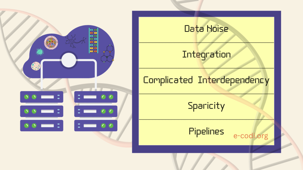
Biological data is unique in several ways:
- It is often high-dimensional, where the number of features (genes, proteins) exceeds the number of samples.
- It is noisy, as biological systems inherently vary between cells, tissues, and individuals.
- It may be sparse, especially in single-cell datasets, where many genes are zero in most cells.
- It is interdependent, since biological variables often correlate—genes co-express, proteins interact, pathways overlap.
This makes traditional statistical approaches often insufficient. Thus, domain-specific preprocessing, such as normalization, batch effect correction, and dimensionality reduction, becomes critical.
Domain-specific processing means using analysis methods, algorithms, and tools tailored to handle the unique features of biological data.
Now we will discuss these challenges in detail
1. What is Noise in Biological Data?
Data noise in biology refers to the random variation or unwanted signals that can obscure true biological patterns.
Source of data noise: This noise can come from natural biological differences, such as variation between individuals or cells, as well as technical factors like differences in lab conditions, instruments, or sample preparation.
How to find noise in data? To understand noise systematically, researchers often start by visualizing the data using tools like PCA plots or heatmaps to identify outliers or unexpected patterns. Analyzing replicates, both biological and technical, also helps distinguish meaningful signals from random variation.
Once identified, noise can be reduced through normalization techniques and batch effect correction methods. . Common normalization methods include scaling counts to a common total or using transcript-per-million (TPM) for RNA-seq data, while microbiome studies may apply rarefaction or compositional normalization techniques.
By carefully controlling for noise, researchers can ensure that their results reflect genuine biological differences rather than artifacts of the data collection process.
How to Consider Interdependency in Biological Data?
Interdependency of data in biology is highly complex. It means how:
- Cells respond to intercellular signals, etc.
- Genes interact (gene–gene interactions or epistasis),
- Genes and environment interact (GxE),
- Proteins regulate each other (protein–protein interaction networks),
- Microbiome influences host metabolism,
We need to cosider here:
- Suppression or masking (e.g., a signal is hidden until another variable is controlled)
- Synergistic effects (e.g., gene A and gene B have no effect alone, but together they activate gene C)
- Conditional dependencies (e.g., A affects B only if C is active)
To detect these higher-order interdependencies, you can use:
Tree-Based Models
- Use Random Forest or XGBoost.
- Analyze SHAP interaction values to reveal hidden dependencies.
Bayesian Networks
- Model conditional dependencies among variables.
- Tools:
bnlearn(R),pgmpy(Python)
Regression with Interaction Terms
- Include terms like
A:BorA:B:Cin your model to capture interactions.
Deep Learning / GNNs
- Neural networks and Graph Neural Networks can learn complex patterns.
- Use interpretability tools like SHAP or LIME.
Tensor Decomposition
- Useful for high-dimensional or time-series data to capture hidden structures.
Use Prior Biological Knowledge
- Integrate pathway data (e.g., Reactome, STRING) to guide analysis and reduce false discoveries.
Sparcity in Biological Data- Causes and solutions
The first important step is to understand the reasons behind the sparsity. Sometimes, sparsity reflects true biological variation, such as genes not being expressed in certain cells or species absent in some samples. Other times, it is caused by technical limitations like dropouts in single-cell sequencing or insufficient sampling depth. Knowing why the data is sparse helps to decide the best approach to manage it.
Before analysis, preprocessing the data is crucial. This often involves filtering out features or samples that contain too many zeros or very low counts, as these may add noise rather than useful information.
Sometimes, zeros in the dataset represent missing or undetected values rather than true absences. In such cases, imputation methods can help fill in these missing values with likely estimates, improving the quality of downstream analysis. Techniques like k-nearest neighbors imputation or model-based approaches such as scImpute for single-cell RNA-seq are often used, but care must be taken as improper imputation can introduce bias.
Focusing on the most informative features can improve analysis quality as well. Feature selection methods help identify genes or species that contribute the most biological signal, often through variance filtering or differential expression analysis.
Developing Biostatistical and Bioinformatics Pipelines for Data Analysis
A data analysis pipeline is a step-by-step process used to collect, clean, transform, analyze, and interpret data in order to extract meaningful insights or make informed decisions. It organizes the workflow into logical stages, making data handling efficient, reproducible, and scalable.
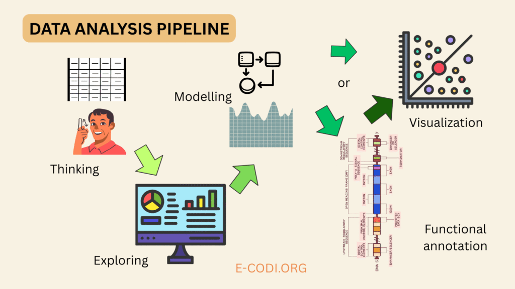
1. Data Understanding and Preprocessing
Before applying any algorithms, one must understand the nature and structure of the data. What is measured? What technology was used? Are there outliers, missing values, or confounders like batch effects or patient sex? For gene expression, this includes raw count normalization (e.g., via TPM or DESeq2’s method).
2. Exploratory Data Analysis (EDA)
Next, researchers use biostatistical methods and visualizations—PCA, t-SNE, clustering—to inspect structure and noise. Outlier detection, transformation (log, variance stabilization), and filtering irrelevant features all help prepare the data.
3. Statistical Modeling
Depending on the hypothesis, researchers apply statistical tests or models. In multi-group studies, this includes generalized linear models (GLMs), mixed models, or survival analysis. For omics data, FDR-adjusted p-values are calculated using methods like Benjamini-Hochberg.
4. Functional Annotation and Enrichment
Once differentially expressed genes or variants are identified, bioinformatics pipelines often include functional enrichment analysis using databases like GO, KEGG, or Reactome. This helps link statistical results back to biology.
5. Visualization and Reproducibility
Creating plots that reveal biological meaning is a crucial part of the pipeline. Tools like ggplot2 (R) or Seaborn (Python) are used for customizable, publication-ready graphics. Reproducibility is enforced using Jupyter Notebooks, RMarkdown, Git, and workflow engines like Snakemake or Nextflow.
Data Integration and Multi-Omics Challenges
One of the most pressing challenges in biological data analysis is integration—combining data from multiple omics levels (genomics, transcriptomics, proteomics, metabolomics) to create a holistic view of biology.
However, integration is difficult because:
- Data scales differ (counts vs. concentrations)
- Measurement noise varies by omics platform
- Sample sizes are limited, especially for rare diseases
- Temporal resolution may mismatch between datasets
To address these issues, researchers use methods like:
- Matrix factorization (e.g., MOFA, iCluster)
- Bayesian hierarchical models that account for noise and scale
- Graph-based integration, where omics data are represented as nodes and edges in biological networks
- Deep learning autoencoders, which can reduce each omic into a latent space, then merge those spaces
One popular approach is matrix factorization, which breaks down large data matrices into smaller, interpretable components. This helps uncover shared patterns across datasets by representing each dataset as a product of latent factors. By doing this, matrix factorization reduces data complexity and highlights underlying biological signals common to multiple data types.
The goal is always to preserve biological signal, reduce redundancy, and increase interpretability.
Conclusion: A Future Powered by Biological Data Science
The frontier of biology is computational. Whether one is decoding gene regulation, modeling immune responses, or predicting patient outcomes, data analysis underpins all modern discoveries.
To succeed, biologists must move beyond wet-lab intuition and embrace pipelines built with biostatistics, bioinformatics, and multi-omics integration. This doesn’t mean becoming a computer scientist—but it does mean mastering the workflows, tools, and reasoning behind data-driven biology.
In the coming years, breakthroughs will rely not just on better experiments, but on sharper algorithms, cleaner data, and smarter integration strategies.
If you like the article, follow E-CODI and share with others !
Bonus Info !
Predictive biology is a subfield that uses data science, mathematical modeling, and machine learning to forecast biological outcomes based on patterns in existing data. For example, predictive models can estimate disease risk from genetic data, simulate protein folding, or predict how ecosystems will respond to climate change. Instead of merely describing biology, predictive biology aims to anticipate behavior and make informed decisions, such as identifying drug targets or engineering biological systems. As biology becomes increasingly data-intensive, predictive approaches are reshaping how biologists conduct research, solve problems, and develop applications in health, agriculture, and the environment.
Pingback: Decoding Regression Models in Biostatistics: A Simple Guide - E.CODI