Understanding Microbiota Data from 16S rRNA Sequencing: What It Is and How to Analyze It

Microbiota research is booming, helping scientists understand how microbes affect health, disease, and the environment. One of the most common techniques to study microbial communities is 16S rRNA sequencing. If you’ve just received microbiota data—or are about to—here’s a simple guide to what it looks like, how it’s generated, and how to make sense of it.

What is 16S rRNA Sequencing?

16S ribosomal RNA (16S rRNA) is a component of the 30S small subunit of prokaryotic ribosomes (like in bacteria and archaea). It’s a ribosomal RNA molecule, not a protein, and it plays a critical role in protein synthesis.

The 16S ribosomal RNA gene is present in almost all bacteria. It contains both highly conserved and variable regions, making it perfect for identifying bacteria at the genus or species level.

Instead of sequencing entire genomes (which is done in shotgun metagenomics), 16S sequencing targets just this one gene. It’s cheaper, faster, and gives a good snapshot of who’s there in a microbial community—like the gut, soil, or water.

What Does the Data Look Like?

When you receive raw data from a 16S sequencing project, it usually includes:

1. FASTQ files

• These are the raw sequencing reads.
• Usually paired-end: two files per sample (e.g., sample1_R1.fastq.gz, sample1_R2.fastq.gz).

A fastq.gz file is a compressed FASTQ file used in bioinformatics to store DNA or RNA sequencing data.

A FASTQ file stores raw sequencing reads from machines like Illumina.

Each sequencing read in a FASTQ file has 4 lines:

1. Line 1: Sequence ID (starts with @)
2. Line 2: DNA sequence (A, T, C, G, N)
3. Line 3: A + symbol (can optionally repeat the ID)
4. Line 4: Quality scores (in ASCII characters)

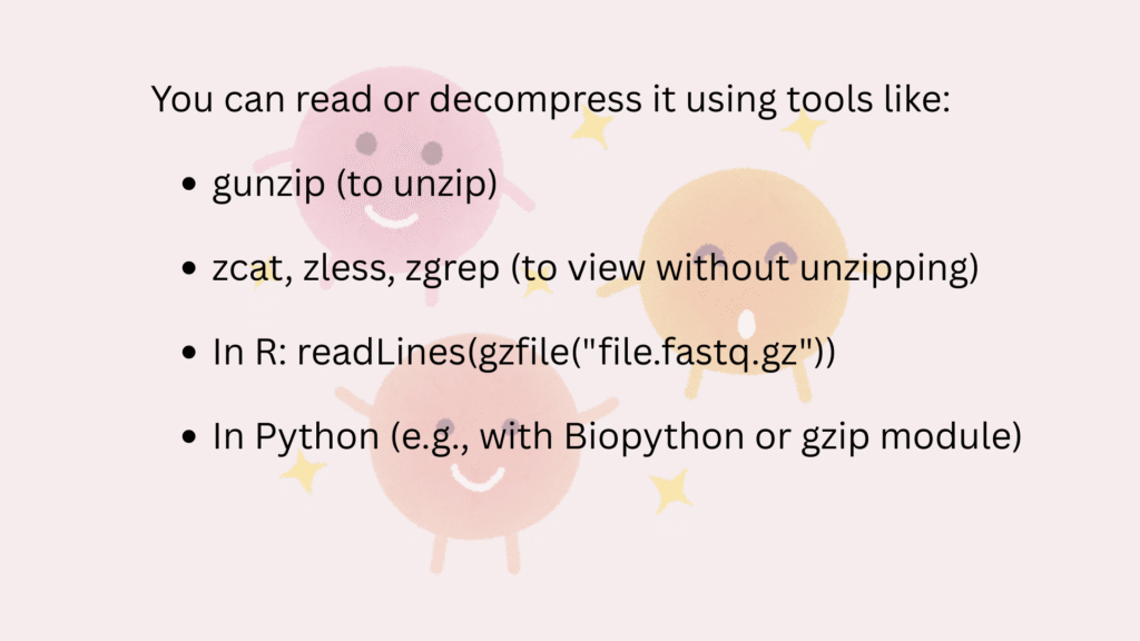
.gz = GZIP compressed

• FASTQ files are usually large, so they are compressed using GZIP.
• A fastq.gz file is smaller and faster to transfer or store.

What Is a Paired-End File?

• They can be large—hundreds of MBs to several GBs, depending on the number of samples and depth.

2. Metadata file

• A spreadsheet (.csv or .tsv) with information about each sample.
• Columns might include: SampleID, Treatment, Timepoint, Host, Location, etc.

What are Steps To Handle 16S Data?

Raw Data (.fastq.gz)
    ↓
Quality Control
    ↓
Filtering and Trimming
    ↓
Denoising (ASV) or Clustering (OTU)
    ↓
Taxonomic Classification
    ↓
Diversity Analysis & Visualization

OTU vs ASV – Two Type of 16S data

Feature	OTU (Operational Taxonomic Unit)	ASV (Amplicon Sequence Variant)
Definition	Cluster of similar sequences (e.g., 97%)	Exact sequence variants (single-nucleotide resolution)
Approach	Clustering	Error correction + inference
Tools	QIIME 1, UPARSE, mothur	DADA2, Deblur
Reproducibility	Low	High
Resolution	Lower (species level)	Higher (species or even strain level)
Recommendation	Legacy method	Modern standard

Use ASVs unless you have specific reasons to use OTUs.

OTU and ASV in Detail

Example to Understand:

Imagine you sequence a sample and get these five sequences:

1. ATCGTACGAT
2. ATCGTACGAT
3. ATCGTACGTT
4. ATCGTACGAT
5. ATCGTACGAT

• OTU method: “Most of these are 97% similar → put them in the same OTU.”
• ASV method: “There are two unique real sequences here → one is ATCGTACGAT, and the other is ATCGTACGTT.”

In modern metagenomics, we often use ASVs (Amplicon Sequence Variants) instead of OTUs (Operational Taxonomic Units) to describe microbial diversity. OTUs group reads based on a similarity threshold (like 97%), which can lump together slightly different sequences. ASVs, on the other hand, represent exact sequences after quality control and error correction, giving much higher resolution and reproducibility. By using ASVs, we can detect subtle differences between microbial communities that OTUs might miss, leading to more accurate diversity estimates and clearer ecological insights.

What is Quality Control (QC) in 16S?

Quality control means checking your DNA reads for errors, trimming bad parts, and keeping only the good, clean sequences. Sequencing machines (like Illumina) sometimes produce:

• Low-quality bases (especially near the ends)
• Adapters (non-biological extra sequences)
• Chimeras (fake sequences formed by two merged reads)
• Short or too long reads
• Sequencing errors (wrong nucleotides)

If you don’t clean your data, you’ll get false bacteria, wrong diversity results, and misleading conclusions.

Common Quality Problems

Problem	What It Means
Low base quality	Some nucleotides are uncertain (bad score)
Adapter contamination	Sequencing machine added extra unwanted pieces
Chimeras	Two real sequences accidentally joined
Short reads	Truncated, often unusable
Duplicates	Technical repeats, not real biological repeats

Key Quality Parameters to Check

Parameter	What You Look For	Common Threshold
Phred score (Q)	Base call quality	≥ Q30 is good (error rate ≤ 1 in 1000)
Read length	After trimming, still long enough	≥ 200 bp is often acceptable
GC content	Consistent with expected	~40–60% typical for bacteria
Adapter presence	Remove all	0% remaining
Chimera rate	Should be low	<5% ideally

How to Do QC (Short Version)

Step 1: Inspect Raw Reads

Use tools like:

• FastQC (visual report of base quality, length, GC%, etc.)

• MultiQC (combine reports if you have many samples)

Step 2: Trim and Filter

Use tools like:

• Trimmomatic, Cutadapt, or fastp for trimming adapters and low-quality bases.
• In DADA2, trimming and filtering are built-in (filterAndTrim()).

Step 3: Denoise and Remove Chimeras

• Use DADA2 or Deblur to:
  • Model and correct sequencing errors
  • Remove chimeras with removeBimeraDenovo()

Taxonomic Classification in 162 Data

After generating ASVs (or OTUs), you now want to know which bacteria those sequences represent. Taxonomic classification assigns each sequence to a level like:

• Kingdom → Bacteria
• Phylum → Proteobacteria
• Class, Order, Family, Genus, and maybe Species

You go from a DNA sequence to a biological name using a reference database.

How does it work?

• The program compares each ASV sequence to a known reference database of bacterial 16S sequences.
• It finds the best match and assigns the most likely taxon (e.g., Genus: Lactobacillus).
• If a perfect match isn’t found, it may assign a higher level (like Family or Order).

Common Databases:

• SILVA (very complete, updated)
• Greengenes (older, but fast)
• RDP (easy for teaching)

Easy R Workflow with DADA2:

taxa <- assignTaxonomy(seqtab.nochim, "silva_nr99_v138.fa.gz", multithread=TRUE)

Diversity Analysis

Now that you know what bacteria are in each sample, it’s time to ask:

• How many kinds of bacteria are there?
• Are two samples similar or different in bacterial composition?

This is diversity analysis.

There are two types:

1. Alpha Diversity – diversity within a single sample
2. Beta Diversity – diversity between different samples

Alpha Diversity: How Diverse Is One Sample?

Alpha diversity gives you an idea of how rich and even a single microbiome sample is.

There are two aspects:

• Richness = How many different species (or ASVs/OTUs) are present?
• Evenness = How evenly are these species distributed?

🔹 1. Shannon Diversity Index

• Balances richness and evenness.
• Sensitive to rare species.

Interpretation:

• Higher values = more diverse and balanced communities.
• A sample with many species but dominated by one will have a lower Shannon score.

Simpson’s Index

• Focuses more on dominance than rare species.
• Measures the probability that two randomly selected individuals belong to the same species.

• Interpretation:
  • Closer to 0 → low diversity (one species dominates)
  • Closer to 1 → high diversity

Tools in R for Alpha Diversity:

• phyloseq::estimate_richness()
• vegan::diversity()
• Visualize with boxplots using ggplot2

Beta Diversity: How Different Are Two Samples

Beta diversity compares microbial composition between samples, helping you understand community structure shifts due to environment, health, treatment, etc.

1. Bray-Curtis Dissimilarity

• Considers both presence and abundance of taxa.
• Measures how different two samples are in terms of shared species.
• Ranges from:
  • 0 = completely similar
  • 1 = completely different
• Visualized with:
  • PCoA plots (Principal Coordinates Analysis)
  • NMDS plots (Non-metric Multidimensional Scaling)
• Tools in R:
  • vegan::vegdist()
  • phyloseq::distance()
  • Plot with phyloseq::plot_ordination() or ggplot2

---

🎯 Which Diversity Metrics to Use?

Goal	Use	Reason
Richness only	Chao1, Observed ASVs	Just counts species (no evenness)
Balanced richness & evenness	Shannon	Popular, robust for most applications
Dominance focused	Simpson	Highlights if few species dominate
Sample comparison	Bray-Curtis	Abundance-sensitive comparison across samples
Presence/Absence only	Jaccard	Ignores abundance;

Metagenomics begins with raw sequencing reads stored in FASTQ files, which contain both the DNA sequences and their quality scores. Before any real analysis, these reads must be checked and cleaned using quality-control tools like FastQC and trimming programs to remove low-quality bases and adapters. Once the data are reliable, the sequences can be assigned to taxa or assembled into longer contigs, turning millions of short reads into information about which organisms are present. From these taxonomic profiles, diversity metrics such as richness, Shannon index, or Bray–Curtis dissimilarity can be calculated to show how varied and balanced the microbial communities are within and between samples. In short, metagenomics data handling moves step by step from raw FASTQ files, to quality scoring, to diversity calculations—transforming raw DNA reads into meaningful ecological and biological insights.